Showing posts with label software. Show all posts

Saturday, April 12, 2014

Cook Your Own Raw Files, Part 3: Demosaic Your Images

AS SOON AS I wrote the following lines at the end of the last article in this series, I regretted it; I wasn't sure why, but I had a nagging feeling that it was too dismissive:
Logically, I am presenting demosaicing as the first step in processing a raw file, but this is not necessarily the best thing to do — I am simply describing it now to get it out of the way.
The article is Cook Your Own Raw Files, Part 2: Some Notes on the Sensor and Demosaicing.

By trying to “get it out of the way,” perhaps I wasn't thinking about my readers, who might get something out of attempts to do demosaicing themselves. It is an important process that goes on in the camera, something that needs to be done right. The purpose of this series is to demonstrate the various steps that a digital camera or raw processor might go through in producing an image, for the education of photographers and retouchers. Simply omitting an important step because it is difficult is not helping anyone.

In the first article in the series, Cook Your Own Raw Files, Part 1: Introduction, I mentioned that I use Raw Photo Processor to produce lightly-processed images that can be used to experiment with the kinds of processing that goes on in raw converters. But this is a Macintosh-only application; and so, for users of Windows, Linux, and other computer operating systems I suggested using dcraw, but I hardly knew much about it.

But I recently discovered that dcraw can produce undemosaiced images; while this is in the documentation, I overlooked it. This feature can allow interested persons the ability to easily try out the demosaicing process themselves. You can get your own free copy of dcraw at http://www.cybercom.net/~dcoffin/dcraw/; it is a command-line utility, which makes its use more difficult for those computer users only familiar with typical graphical interfaces, but a bit of effort in trying this out can be worthwhile. The command to convert a file is thus:

dcraw -v -E -T -4 -o 0 DSC_5226.NEF

Where ‘DSC_5226.NEF’ is the camera raw file that you want to convert. You must issue the command in the same directory or folder where the file is located, or otherwise supply a path to the file. The command will output a TIFF file in the same directory: in this instance, dcraw will output DSC_5226.tiff.

The options used have this meaning:
  • -v Verbose output — the command will display extra text which might be useful in our further processing.
  • -E Image will not be demosaiced; also, pixels along the edges of the sensor, normally cropped by the camera, are retained.
  • -T Output an image conforming to the Tagged Image File Format (TIFF) is output. Many common image editors can read these lossless files.
  • -4 A 16-bit image is produced instead of the more common 8 bit image files, which gives us more accuracy, without any gamma conversion or white level adjustments. This gives us a dark, linear image.
  • -o 0 This is a lower-case letter ‘o’ and a zero. This turns off the adjustment of colors delivered by the camera; this option will deliver uncalibrated and unadjusted color.
These settings will give us an image file which most closely represents the raw data delivered by the camera. Also, I ought to note that a white balance won't be done by dcraw, turning off the mechanism which compensates for the color of the light illumining the scene in the image.

Here is a view of some bookshelves in my office, from approximately the same angle of view that I see from my computer:
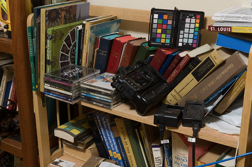
Messy bookshelf - Adobe Camera Raw developed

The color and tonality in this photograph on my calibrated monitor look pretty close to what I see in real life — maybe some of the bright yellows are a bit off. Otherwise this is a suitable image taken with reasonably good gear and technique. I will use this image as the sample for our further processing in this article. You can get a copy of this original Nikon raw NEF file here.

OK, I ran this image through dcraw using the settings shown above, and I get this result:
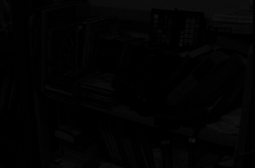
DSC_5492 - undemosaiced

Not much to see here! If we take a closer look at the file:

DSC_5492 - undemosaiced, detail

We can see that it is monochrome, extremely dim, and has the camera's mosaic pattern on it. You can download a copy of this processed file here.

The image is so dark partly because my Nikon delivers 14 bit raw images — while the image format itself is 16 bits, and so we have unused brightness numbers. If you are unfamiliar with bits, you might want to review the Wikipedia article on binary numbers. Basically, the number of bits in this case is a measure of how many levels of brightness is represented in the raw file. If you add one bit of depth to an image, you double the number of levels of brightness:
  • If you have a one bit-depth image, you only have two levels of brightness — white and black.
  • In a two bit image, you have four levels of brightness — black, dark gray, light gray, and white.
  • Three bits gives 8 levels, four bits give 16 levels, five gives 32 and so forth.
  • A 14 bit image has 16,384 levels, and a 16 bit image has 65,536 levels.
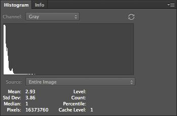
Each additional bit doubles the number of levels, and since my camera has 14 bits, it has one quarter the number of brightness levels that can be found in a 16 bit image. Since the dcraw command delivered a linear image — where ‘linear’ means that a pixel with double the exposure will have double the brightness number — we can correct for the camera's lack of a full 16 bits by using the Levels tool in Photoshop. Here is the original histogram of the image:

Original histogram of DSC_5492

When we process an image, we need to use all of the 16 bits, because white is defined as the brightest 16 bit number.

Understand that with a linear image such as this, the entire right half of the histogram is brightness levels associated with the 16th bit; and half of what is left is data associated with the 15th bit. So to scale the 14 bits data we have, so as to use all 16 bits, we can chop off the part of the data that isn't used by Nikon — the top three quarters of the histogram. Photoshop's Levels tool only gives us the ability to adjust 256 levels of brightness — 0 is black and 255 is white — even when working with a 16 bit file, but for our purpose this isn't a problem. So the 16th bit takes up the upper half of the data, the top 128 levels, from 128 to 255, while the 15th bit takes up the range from 64 to 127.

So for a 14 bit camera, we need to set levels to 63:
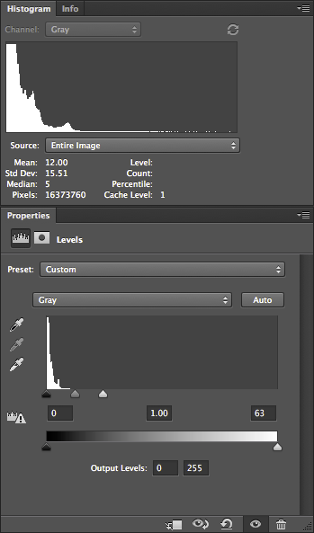
Corrected histogram and levels of DSC_5492

This use of Levels gives us the same results as if we multiplied all of our image numbers by 4.

Notice how the histogram shows that there is some image data going all of the way across — although, for other reasons, often won't quite touch the right hand side. Be aware that linear images tend to have most of their data clustered around the darkest, or lefthand part of the histogram — this is normal. JPEGs delivered by cameras, or images viewed on the Internet, have a gamma correction applied to them, which is a kind of data compression that assigns more color numbers to shadows and mid-tones at the expense of highlights. This actually works out well, but adds mathematical complexity, which I hope to cover later. This will give us a nice, usable histogram where most of the values are typically clustered around the middle instead of way down at the left hand edge.

Many cameras are 12 bit, and so the Levels would have to be set at 15 — which would give us the same results that we would get by multiplying all of the values in the image by 16.
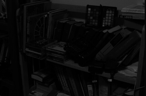
DSC_5492 - undemosaiced, scaled

Our image is now brighter and we can actually see the subject tolerably well.

Now Photoshop is hardly the best software to do demosaicing, but it can be done with many cameras. The first thing we need to do is to identify the mosaic pattern used by the camera— there are a wide varieties of patterns used in the industry, but fortunately, there are a few that are commonly used. One major exception is Fuji, which often uses innovative patterns in their cameras. Sigma, which uses Foveon X3 sensors, do not have a pattern, and so this entire discussion on demosaicing is irrelevant.

My Nikon camera uses the RGGB pattern, where, starting in the upper-left hand corner of the image, we have a pattern that looks like this:
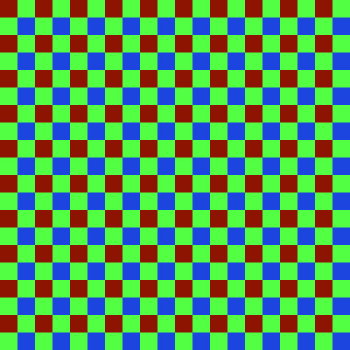
Array

We have a repeating pattern of 2x2 blocks, with red in the upper left hand corner, and blue in the lower right hand corner.

You will have to look up the pattern used in your camera, or simply use my example files linked above. If you have clever computer programming skills, you might even be able to parse the dcraw.c source code for clues — all of the supported camera patterns are encoded in the file. However, be aware that not all mosaic patterns can be decoded by my method, which assumes the RGGB pattern. However, if your camera pattern is a rotation of this, you might be able to rotate your image to get it to fit — for example, I demosaiced a Panasonic camera raw file, which has a BGGR pattern, simply by rotating the image 180 degrees.

First duplicate the undemosaiced file in Photoshop, and convert it to the standard sRGB IEC61966-2.1 color space. The color space isn't yet important, but it will help you see what is going on in the processing. Now this conversion will mess with the tonality of image, and so I select each of the three color channels separately, and do an Image->Apply Image… command to put the original grayscale values into the new RGB image.

Then I create a 2x2 pixel image which duplicates the array pattern:


You see that little dot, right? That is the 2x2 image. Here is a bigger version:
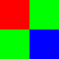
rggb pattern - large

Then I select the menu Edit, then Define Pattern…, then give it name.

On the new image, I create a new layer, go to Edit, then Fill… and then Use: Pattern, and then select my new Custom Pattern. The new layer will be filled with the repeating mosaic pattern. I turn this layer off so we don't have to see it.

Then I duplicate the image into three layers, which I name red, green, and blue, and put a layer mask on each.

On the red layer mask, I apply the red channel of the color pattern, using Image, Apply Image…:
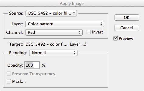
Apply pattern mask

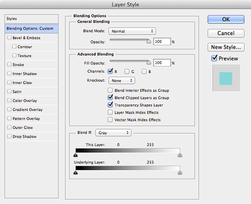
This gives us only the red bits of the color filter array in this layer. I do the similar action for the other layers. Then, I double click on the layer name in the Layers tab, and this comes up:
Layer style

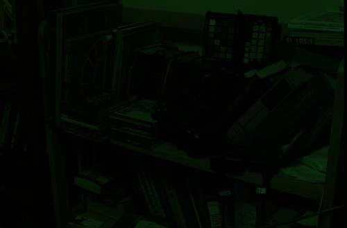
I select only the R channel, unchecking G and B; this turns the layer into the red color, and then I do the same for the blue and green layers, selecting only the corresponding channel to the layer. When I fill the bottom original layer with black, this results:
DSC_5492 - color filter array

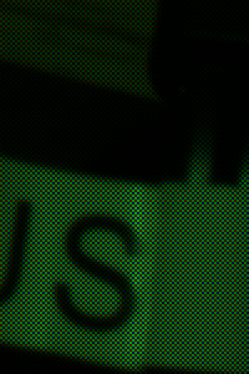
It appears to be a full-color image, albeit with a very bad white balance; but if we examine a small part of it:
DSC_5492 - color filter array, detail

We can see the color filter array on the image. You can download the full color mosaic image here.

The demosaicing procedure I will show here is completely ad hoc, but at least it might give Photoshop owners some of the flavor of the process. You might want to review the article Cook Your Own Raw Files, Part 2: Some Notes on the Sensor and Demosaicing for an overview of the process.

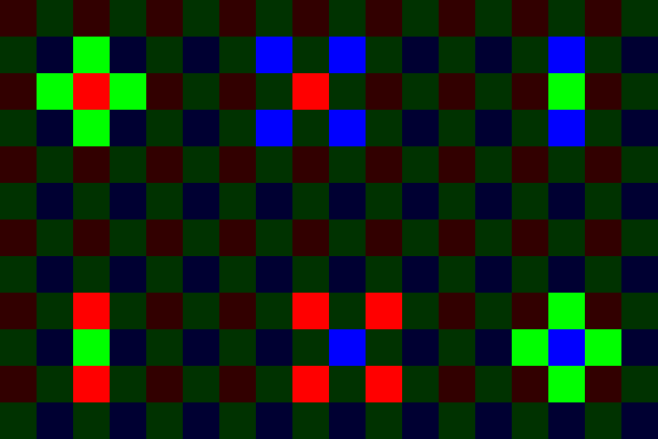
The basic problem is this — at any given pixel location, we only have one color, and we have to estimate the other two colors, based on the colors found in surrounding pixels. So for each type of pixel in our color array, we need need two functions to get the color, which for our 2x2 matrix, gives us 8 functions. For this exercise, I'll use a bilinear function, which is pretty good although still being simple.

Following is an illustration of bilinear demosaicing functions, which takes averages of all the adjacent surrounding pixel values to estimate full-color at each pixel.
Bilinear-demosaic-animation

In order to do demosaicing in Photoshop, we can use the obscure Custom filter, found in the menus under Filter->Other->Custom…

We will have to use four custom filters for this task, corresponding to the four types of patterns seen in the above animation:
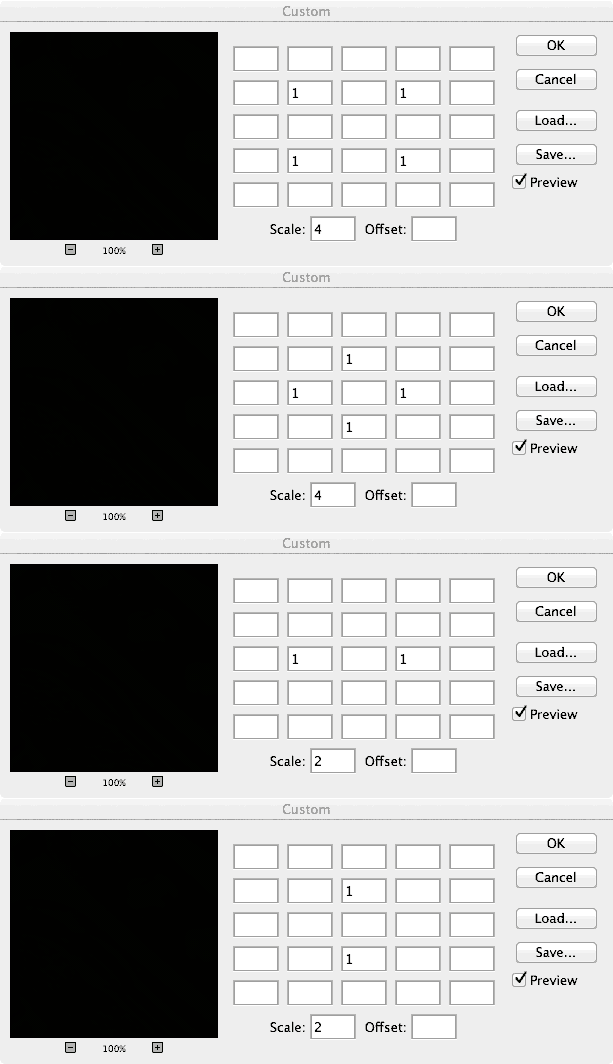


An explanation of the Custom Filter function can be found here.

We will now create a complex layered file, with a layer for each of our eight color estimates. The key to using this — since Custom Filter changes all pixels — is to use masking to limit our processing to solely red, green, and blue pixels where appropriate.

Here are the layers in the file:
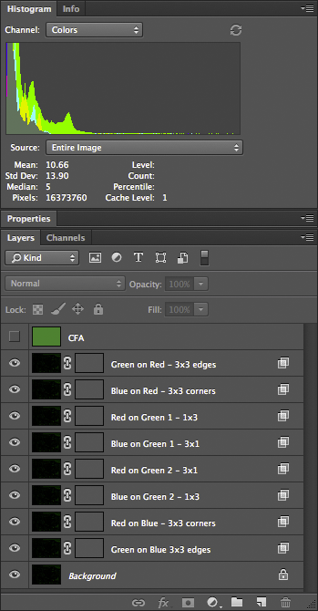
Demosaic layers

Doing this right requires a bit of patience and diligence. I named the layers to help do this more accurately. All of these layers, at first, are simply duplicates of our color mosaic image. The top layer is the color mosaic array, created using custom patterns — we will use this to create our masks.

The next layer — Green on Red - 3x3 edges — is processed like this:
  • We are estimating green color values for our red pixels; using the Layer Style (the box is opened by double-clicking the layer) we restrict this layer to only the green channel — G is selected in the Layer Style box.
  • Likewise, for all the rest of the layers, we restrict the color channel to whatever color is being estimated: B for Blue on Red, G, for Green on Blue, etc.
  • The masks, however, correspond to the color in the mosaic. For Green on Red, we are restricting processing to only the red pixels, giving them a green value in addition to red.
  • The CFA layer is useful for creating these masks; for example, for the Green on Red layer, I used Image->Apply Image, selecting the Red channel of the CFA layer, applying it to the layer mask. This gives us a mask where only the red matrix colors are visible.
  • If you zoom way into the image, so far nothing has changed; but the custom filter will alter the image. I used the custom filter indicated by the layer name. For the Green on Red layer, I used the 3x3 edges filter — which averages the four green pixels found on the edges of the red pixels, and then assigns that average to the green channel of the red pixel. These custom filters can be found here.
  • The two green pixels are handled separately. What I do is use the Red or Blue channel from the CFA layer as a mask, and then shift it by one pixel according to the location, using Filter->Other->Offset; and I set it to Wrap Around.
When setting up these layers, you might want to record an action so that you can do this repeatedly with little effort. Also remember that using the bilinear demosaicing algorithm will leave a border around the edges of the image.

Once all the layers are set up, we have a nicely demosaiced image:

DSC_5492 - demosaiced

You can download the 16-bit file here. A version of the file, with all of the layers, can be found here; beware, however, it is over half a gigabyte in size.

Looking more closely:
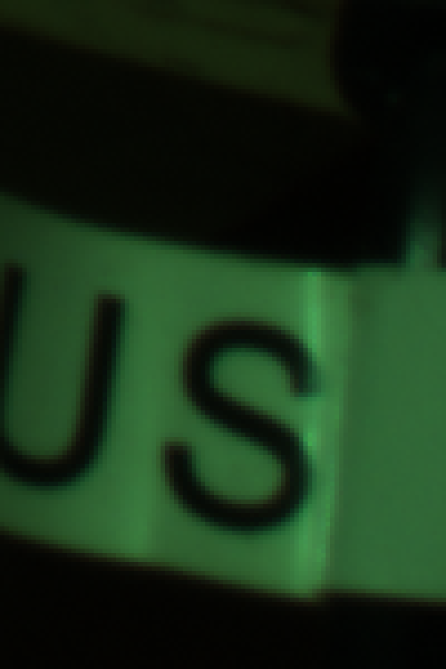
DSC_5492 - demosaiced - detail

It appears that the demosaicing process was pretty clean; there might be some color fringing here, but I think most of it is chromatic aberration from the optics.

The next process is removing this color cast by doing a white balance. However, just because we are logically doing demosaicing first, this does not mean that this is optimal for getting good image quality — perhaps we might want to do white balance before demosaicing.

Obviously, it is a bit silly doing demosaicing in Photoshop — but it does work in this case — although a general-purpose programming language would be better.

Other articles in the series are:

Cook Your Own Raw Files, Part 1: Introduction
Cook Your Own Raw Files, Part 2: Some Notes on the Sensor and Demosaicing

Saturday, March 8, 2014

Cook Your Own Raw Files, Part 2: Some Notes on the Sensor and Demosaicing

ADMITTEDLY, DIGITAL cameras are somewhat difficult to characterize well, because there is so much variety between models, but there are a few simple measures to help. Likely, most digital camera users are familiar with the term megapixels — perhaps with the vague understanding that more is better, but like many things, there is some sort of trade-off. Unfortunately, a particular megapixel value is usually hard to directly compare to another, simply because there are other factors we have to consider, like the sharpness of lenses used, the size of the sensor itself, any modifications made to the sensor, the processing done on the raw image data by the camera’s embedded computer, and a multitude of other factors. A 12 megapixel camera might very well produce sharper, cleaner images than a 16 megapixel camera.
This is the second article in a series; the first article is here:
Cook Your Own Raw Files, Part 1: Introduction
It is important to know is that there are a fixed number of light-recording sites on a typical digital camera sensor — millions of them — which is why we talk about megapixels. But consider that for many uses, such large numbers of pixels really aren’t needed:

Building in Soulard

A building in the Soulard neighborhood, in Saint Louis, Missouri, USA.

By modern standards, this is a very small image. It is 500 pixels across by 332 pixels in height; and if we multiply them together, 500 x 332 = 166,000 total pixels. If we divide that by one million, we get a tiny 0.166 megapixels, a mere 1% or so of the total number of pixels that might be found in a contemporary camera. Don’t get me wrong — all the extra megapixels in my camera did find a good use, for when I made this image by downsampling, some of the impression of sharpness of the original image data did eventually find its way into this tiny image — if I only had a 0.166 megapixel camera, the final results would have been softer.

OK, it is very important to know that a digital image has ultimately a fixed pixel size, and if we enlarge it, we don’t get any more real detail out of it, and if we reduce it, we will we lose detail. Many beginners, if they get Photoshop or some other image editing software, will get confused over image sizes and the notorious “pixels per inch” setting, as we see in this Photoshop dialog box:

Image Size Dialog Box

If you are displaying an image on the Internet, the “Resolution” or “Pixels/Inch” setting is meaningless because the image will display on the monitor at whatever the resolution of the display happens to be set at. Likewise, if you make a print, the Width and Height values you see here are likewise meaningless, for the dimensions of the printed image will be whatever size the image is printed at — and not these values. But — if you multiply the Pixels/Inch value by the Width or Height, you will get the actual pixel dimensions of the image.

The really important value then is the pixel dimensions: my camera delivers 4928 pixels across and 3264 pixels in the vertical dimension. I can resample the image to have larger pixel dimensions, but all those extra pixels will be padding, or interpolated data, and so I won’t see any new real detail. I can resample the image smaller, but I’ll be throwing away detail.

Sensels and Pixels

So, we might assume that my camera’s sensor has 4,928 pixels across and 3,264 pixels vertically — well, it actually has more than that, for a reason we’ll get to later. But in another sense, we can say that the camera has fewer pixels than that, if we define a pixel as having full color information. My camera then does not capture whole pixels, but only a series of partial pixels.

It would be more correct to say that a 16 megapixel camera actually has 16 million sensels, where each sensel captures only a narrow range of light frequencies. In most digital cameras, we have three kinds of sensels, each of which only captures one particular color.

The image sensor of my particular model of Nikon has a vast array of sensels — a quarter of which are only sensitive to red light, another quarter sensitive to blue light, and half sensitive to green light, arrayed in a pattern somewhat like this one:

Array

Since I was unable to find a good photomicrograph of an actual camera sensor, this will have to do for our needs — but this abstract representation doesn’t really show us the complexity of sensors.

Not only is the sensor most sensitive to a bright yellowish-green light (as far as I can tell), it has less sensitivity to blue, and is less sensitive to red: this is on top of the fact that we have as many green sensels as we have red and blue combined. Please be aware that the camera can only deliver these colors (in a variety of brightnesses), and so somehow we are going to have to find some means of combining these colors together in order to get a full gamut of color in our final image.

We have information on only one color at each sensel location. If we want to deliver a full pixel of color at each location, we need to use an interpolation algorithm — a method of estimating the full color at any particular sensel location based on the surrounding sensels. This process of estimating colors is called demosaicing, interpolation, or debayering — converting the mosaic of colors to a continuous image.

Camera raw files are of great interest because they record image data that have not yet been interpolated; you can, after the fact on your computer, use updated software that might include a better interpolation algorithm, and so you can possibly get better images today from the same raw file than what you could have gotten years ago.

Please be aware that the kind of pattern above — called a Bayer filter, after the Eastman Kodak inventor Bryce Bayer (1929–2012) — is not the only one. Fujifilm has experimented with a variety of innovative patterns for its cameras, while the Leica Monochrom has no color pattern at all, since it shoots in black and white only. Also be aware that the colors that any given model of camera captures might be somewhat different from what I show here — even cameras that use the same basic sensor might use a different color filter array and so have different color rendering. Camera manufacturers will use different formulations of a color filter array to adjust color sensitivity, or to allow for good performance in low light.

Sigma cameras with Foveon X3 sensors have no pattern, since they stack three different colors of sensels on top of each other, giving full-color information at each pixel location. While this may seem to be ideal, be aware that this design has its own problems.

A Clarification

I am using the term ‘color’ loosely here. Be aware that many combination of light frequencies can produce what looks like — to the human eye — the same color. For example, a laser might produce a pure yellow light, but that color of yellow might look the same as a combination of red and green light. This is called metamerism, and is a rather difficult problem. There are any number of formulations of color filters that can be used in a digital camera, and we can expect them to have varying absorbance of light — leading to different color renderings. For this reason, it is difficult to get truly accurate colors from a digital camera.

A Perfect Sample Image

For my demonstrations of demosaicing, I’ll be using sections of this image (Copyright © 2001 by Bruce Justin Lindbloom; source http://www.brucelindbloom.com):

DeltaE_8bit_gamma2.2

Mr. Lindbloom writes:
In the interest of digital imaging research, I am providing a set of four images that represent "perfect" images, that is, they represent a natural scene (as opposed to say, a test pattern or a gradient) which is completely void of any noise, aliasing or other image artifacts. They were taken with a virtual, six mega-pixel camera using a ray tracing program I wrote myself. The intensity of each pixel was computed in double precision floating point and then companded and quantized to 8- or 16-bits per channel at the last possible moment before writing the image file. The four variations represent all combinations of 8- or 16-bits per channel and gamma of 1.0 or 2.2. I believe these images will be useful for research purposes in answering such questions as "How many bits are needed to avoid visual defects?" and "How does one determine the number of bits of real image information, as opposed to digitized noise?" In this sense, they may provide ideal image references against which actual digitized images may be compared by various visual or statistical analysis techniques.
No camera — at the same resolution — will produce images as sharp as this, nor will any camera produce colors as accurate as this image, and no camera image will be without noise. Using perfect images for our purposes has the benefit that it will make defects more visible; real cameras will have less pristine images.

I am using two small crops of this image, 100x150 pixels in size each, which I show here enlarged 500%:

Sample 1

Sample 2

Applying the Mosaic

The sample image has brilliant, saturated colors of impossible clarity. But what happens if we pretend that this image was taken with a camera with a Bayer filter? Here I combine the image crop with a red-green-blue array similar to the one shown above:

Sample 1 mosaic

It looks rather bad, and recovering something close to the original colors seems to be hopeless. What is worse, we apparently have lost all of the subtle color variations seen in the original image. If we take a closer look at this image:

Sample 1 mosaic magnified

We see that we have only three colors [technically the red, green, and blue primary colors of the sRGB standard] with only variation in brightness. We seemed to have lost much of the color of our original image.

But this is precisely what happens with a digital camera — all the richness and variety of all the colors of the world get reduced down to only three colors. However, all is not lost — if we intelligently select three distinct primary colors, we can reconstruct all of the colors that lay between them by specifying varying quantities of each primary. This is the foundation of the RGB color system. Please take a look at these articles:
Removing the Matrix

Now we have lost color information because of the Bayer filter, and for most digital cameras we simply have to accept that fact and do the best we can to estimate the color information that has been lost. Since each pixel or rather sensel only delivers one color — and we need three for full color — we can have to estimate the colors by looking at the neighboring sensels and making some assumptions about the image. Red sensels need green and blue color data, green sensels lack red and blue data, and blue sensels need red and green.

A very simple method for doing this is the Nearest Neighbor interpolation algorithm, where we grab adjacent sensel colors and use those to estimate the full color of the image. Here is an illustration of a nearest neighbor algorithm:

Example of Nearest Neighbor
Take a look at the three original color channels — in the red, we only have data from the red sensel, and the rest are black — and so we copy that red value to the adjoining sensels. Since we have two different green sensels, here we split the difference between them and copy the resulting average to the red and blue sensels. We end up with a variety of colors when we are finished. Now there are a number of ways we can implement a nearest neighbor algorithm, and these depend on the arrangement of the colors on the sensor, and each one will produce somewhat different results.

Here we apply a nearest neighbor algorithm to our sample images:

Sample 1 - Nearest Neighbor

Sample 2 - Nearest Neighbor

OK, it is apparent that we can reproduce areas of uniform color well, giving us back the colors of the original image. However, edges are a mess. Since the algorithm used has no idea that the lines on the second image are supposed to be gray, it gives us color artifacts. Generally, all edges are rough. Also notice that there is a bias towards one color on one side of an object, and a bias towards another color on the other side of the same object — in the samples, the orange patches have green artifacts on its top and left edges, and red artifacts on its bottom and right edges. This bias makes sense since we are only copying color data from one side of each sensel.

We can eliminate this bias if we replace the Nearest Neighbor algorithm with something that is symmetric. A Bilinear algorithm will examine the adjacent colors on all sides of each sensel, getting rid of the bias. Our sample images here are demosaiced with a bilinear algorithm:

Sample 1 - Bilinear

Sample 2 - Bilinear

OK, a bilinear algorithm eliminates the directional bias of color artifacts, which is good. While the edges are still rough, they do seem a bit softer — which makes sense, since we are taking data from a wider range of sensels, which in effect blurs the image a bit.

Demosaicing algorithms all assume that colors of adjacent pixels are going to be more similar to each other than they are different — and if we cannot make this assumption, then we can’t do demosaicing. Nearest neighbor algorithms assume that all colors in a 2x2 block are basically identical, while the bilinear algorithm assumes that colors change uniformly in a linear fashion. If we sample sensels farther away, we can assume more complicated relationships, such as a power series, and this assumption is built into the bicubic algorithm, which produces smoother results than those illustrated.

More complex algorithms will give us better gradations and smoothness in color, but have the side-effect of softening edges, and so there is research in ways of discovering edges to handle them separately, by forcing colors along an edge to one value or another. Some algorithms are optimized for scanning texts, while others are better for natural scenes taken with a camera. Be aware that noise will change the results also, and so there are some algorithms that are more resistant to noise, but may not produce sharp results with clean images.

As high frame rates are often desired for cameras, complex algorithms for producing JPEGs may not be desired, simply because it will take much longer to process each image — however, this is less of a problem with raw converters on computers, since we can assume that a slight or even long delay is more acceptable.

Notice that our bilinear images have a border around them. Because the bilinear algorithm takes data from all around each sensel, we don’t have complete data for the sensels on the edges, and so there will be a discontinuity on the border of the image. Because of this, cameras may have slightly more sensels than what is actually delivered in a final JPEG — edges are cropped.

We ought not assume that a camera with X megapixels needs to always deliver an image at that size: perhaps it makes sense to deliver a smaller image? For example, we can collapse each 2x2 square of sensels to one pixel, producing an image with half the resolution and one quarter the size, and possibly with fewer color artifacts. Some newer smartphone cameras routinely use this kind of processing to produce superior images from small, noisy high-megapixel sensors. This is a field of active research.

Antialias

Don’t pixel peep! Don’t zoom way into your images to see defects in your lens, focus, or demosaicing algorithms! Be satisfied with your final images on the computer screen, and if you make a large print, don’t stand up close to it looking for defects. Stand back at a comfortable distance, and enjoy your image.

Perhaps this is wise advice. Don’t agonize over tiny details which will never be seen by anyone who isn’t an obsessive photographer. This is especially true when we routinely have cameras with huge megapixel values — and never use all those pixels in ordinary work.

But impressive specifications can help you even if you never use technology to its fullest. If you want a car with good acceleration at legal highway speeds, you will need a car that can go much faster — even if you never drive over the speed limit. If you don’t want a bridge to collapse, build it to accept far more weight than it will ever experience. Most lenses are much sharper when stopped down by one or two stops: and so, if you want a good sharp lens at f/2.8, you will likely need to use an f/1.4 lens. A camera that is tolerable at ISO 6400 will likely be excellent at ISO 1600. If you want exceptionally sharp and clean 10 megapixel images, you might need a camera that has 24 megapixels.

OK, so then let’s consider the rated megapixel count of a camera as a safety factor, or as an engineering design feature intended to deliver excellent results at a lower final resolution. Under typical operating conditions, you won’t use all of your megapixels. As we can probably assume, better demosaicing algorithms might produce softer, but cleaner results, and that is perfectly acceptable. Now perhaps those color fringes around edges are rarely visible — although resampling algorithms might show them in places, and so getting rid of them ought to be at least somewhat important.

My attempts to blur the color defects around edges was not fruitful. In Photoshop, I attempted to use a half dozen methods of chroma blur and noise reduction, and either they didn’t work, or they produced artifacts that were more objectionable than the original flaws. The problem is, once the camera captures the image, the damage is already done: the camera does in fact capture different colors on opposite sides of a sharp edge — a red sensel might be on one side of an edge, and the blue sensel captures light from the other side.

In order to overcome unpleasant digital artifacts, most cameras incorporate antialias filters: they blur the image a bit so that light coming into the camera is split so that it goes to more than one sensel. This process can only be done at the time of image capture, it cannot be duplicated in software after the fact. Since I am working with a perfect synthetic image, I can simulate the effect of an antialias filter before I impose a mosaic.

Here I used box blur, at 75% opacity on the original image data before applying the mosaic: demosaicing leads to a rather clean looking image:


Sample 1 - bilinear - antialias

Sample 2 - bilinear - antialias

Now I could have used a stronger blurring to get rid of more color, but I think this is perfectly adequate. What little color noise that still remains can be easily cleaned up by doing a very slight amount of chroma noise reduction — but it is hardly needed. If I would have used stronger blurring, the residual noise would have been nearly non-existent, but it would also have made the image softer. Note that we still have the border problem, easily fixed by cropping out those pixels.

It is typically said that the purpose of the antialias filter is to avoid moiré patterns, as illustrated in the article The Problem of Resizing Images. Understand that moiré patterns are a type of aliasing — in any kind of digital sampling of an analog signal, such as sound or light, if the original analog signal isn’t processed well, the resulting digital recording or image may have an unnatural and unpleasant roughness when heard or seen. From my experience, I think that avoiding the generation of digital color noise defects due to the Bayer filter is a stronger or more common reason for using an antialias filter. But of course, both moiré and demosaicing noise are examples of aliasing in general, so solving one problem solves the other.

Producing a good digital representation of an analog signal requires two steps: blurring the original analog signal a bit, followed by oversampling — collecting more detailed data than you might think you actually need. In digital audio processing, the original analog sound is sent through a low-pass filter, eliminating ultrasonic frequencies, and the resulting signal is sampled at frequency more than double the highest frequency that can be heard by young, healthy ears — but this is not wasteful but rather essential for high-quality digital sound reproduction. Likewise, high megapixel cameras — often considered wasteful or overkill — ought to be seen as digital devices which properly implement oversampling so as to get a clean final image.

Anti-antialias

There has been a trend in recent years of DSLR camera makers producing sensors without antialias filters. A common opinion of this practice is that it makes for sharper-looking images. Indeed they are sharper looking — compare our images that implement the nearest neighbor algorithm with those which are blurred at the bottom. But is that apparent sharpness due to aliasing — a defect of processing — and isn’t real detail at all?

So in some respects, getting rid of an antialias filter ought to be considered a mistake. Perhaps Nikon realizes this, offering both the D800, which incorporates an antialias filter, and the D800E, which incorporates another filter which cancels out the effect of the antialias filter. But be aware that there is no way to digitally correct for the loss of the antialias blurring step of the original analog signal. Any attempts, after the fact, to correct for the digital aliasing flaws, will inevitably be worse than if the analog signal was blurred to begin with.

However, practically speaking, it is extremely difficult to get a pixel-level sharp image from a high megapixel camera, especially when the camera is a small image format like DSLRs. Optics usually aren’t all that good and excellent optics are often rare. Also, camera shake, poor focus, narrow depth of field, and diffraction will all blur the light hitting the sensor, giving us the analog pre-blur that is needed to produce clean digital images. In this case, elimination of the antialias filter can actually provide truly sharper images — since we don’t want to further blur light that is already blurry enough to avoid artifacts.

Be aware that construction of an antialias filter is rather problematic and they are not necessarily mathematically perfect for the purpose of pre-blurring the analog light signal for the Bayer filter. We do find a wide variation of anti-alias filters in various camera models, with some having the reputation of being too strong than needed.

Some Further Notes

A quick Web search for “demosaicing algorithms” will bring up many scholarly articles regarding the strengths and weaknesses of the various methods of interpolation, but these are rarely of interest to a photographer.

What a photographer needs to know is that the process does exist, and that most of the time, the method used isn’t too particularly important. The results and artifacts produced by demosaicing only become critical to image quality when the photographer is trying to do something extreme — like making tiny crops of an image or producing huge images, where exceptional optics are used with refined technique: where there is a real need to produce the cleanest possible images. This might also be useful if you are using a low-resolution camera with sharp optics. Otherwise, for casual photography, the details of demosaicing are of little value. Sometimes we simply need to retouch out obvious defects, like blurring the color along particularly noxious edges.

Most raw converter software does not give us any choice in demosaicing algorithm. But some that do include Raw Photo Processor, dcraw, darktable, and RawTherapee. The latter is interesting because you can quickly see the results of changing the algorithm used.

Logically, I am presenting demosaicing as the first step in processing a raw file, but this is not necessarily the best thing to do — I am simply describing it now to get it out of the way. The Dcraw tutorial demonstrates that white balance ought to be done before demosaicing, otherwise additional color artifacts might be generated.

Click here for the previous article in the series:

Cook Your Own Raw Files, Part 1: Introduction

And the next article:

Cook Your Own Raw Files, Part 3: Demosaic Your Images

Friday, February 7, 2014

Cook Your Own Raw Files, Part 1: Introduction

“IT MUST BE really simple. When a digital camera’s shutter button is pressed, the camera records the amount of light falling on it, which is written to an image file, which we then can display on a computer monitor or send to a printer.”

Well, no, it isn't quite that simple — in fact, it is quite complex, for reasons including:
  • The physics of light
  • The physiology of human vision
  • The psychology of color
  • How cameras sense light in general
  • How cameras sense color difference
  • Technical trade-offs in camera design
  • The efficiency of image data storage and computer processing of images
  • The industry standards that guide camera manufacturers
For example, this nice image of a butterfly is typical of what we would expect from a digital camera:

DSC_4160

The colors look plausible, we can see lots of highlight and shadow detail, and it is fairly crisp. But this is not how the camera records the image. What the camera records is rather something more like this:

DSC_4160 - raw

This is dark and green. Not at all what we would expect, based on the naïve idea which opened this article. If we were to open this image into Photoshop, adjust the brightness, and subtract out the green color, we still would not have good colors — they would rather be somewhat subdued and have the wrong hue — and the image would still appear to be a bit lackluster and soft. There would also be severe banding or posterization in the shadows — but that is a matter for later. However, an image file such as this will give you a good idea of the performance, characteristics, and the limits of your camera.

The purpose of this proposed series of articles is to cover the basic steps that go on within cameras and raw processing software, and to do so, we are going to use some software that will emulate, at least partly, what happens in raw conversion, and I hope will explain it in an easy-to-understand fashion.

Now this is entirely for educational purposes — what I present here is no substitute for actually using a raw processor — but I hope that my readers will find this interesting to know, and maybe learn a few things which might make them better photographers and retouchers.

What we need for our experimentation is some computer software that will deliver the closest possible approximation of a camera’s raw data, which we can pull into Photoshop or some other image editing program for further investigation. I use Raw Photo Processor — a free download — but this, unfortunately, is only for Macintosh computers, but the dcraw program can be used with most any computer.

If you have a Mac, download RPP from http://www.raw-photo-processor.com. There are a few settings in Raw Photo Processor needed to produce a raw-like image:


If your imaging editor allows you to use a full 32-bit workflow, then you can set RPP to use Raw RGB TIFF 32-bit, which will give you better accuracy and less clipping. Photoshop has limited 32 functionality, but ought to be able to do most of the functions we plan to demonstrate.

An alternative is dcraw, a simple command-line program, by author Dave Coffin, whose mission is to “Write and maintain an ANSI C program that decodes any raw image from any digital camera on any computer running any operating system” and this software is used in many raw converter packages. You can download the software from http://www.cybercom.net/~dcoffin/dcraw, and a good tutorial for using it is found here.

This program operates off of the command line, rather than the more common graphical interface. The command to produce a lightly-processed raw-like image file is this:

dcraw -v -T -4 -o 0 198_0011.nef

where you replace 198_0011.nef with the name of the raw file you want to process. This software will generate a TIFF file in the form 198_0011.tiff. See the dcraw documentation for the usage of the utility and its parameters. This command creates a 16 TIFF file equivalent to what is generated by Raw Photo Processor.

I will demonstrate processing on Photoshop, although equivalent functionality for our purposes is available in other software applications.

You might want to experiment with RPP or dcraw, in order to get a good idea of what kind of image data your camera actually delivers. Here are some things you might want to look at and try:
  • When you attempt to open the image in your image editing software, do you get a warning that your image does not have a profile? If so, assign it sRGB; if not, your software may not be color managed or it may automatically assign the standard sRGB color space — but this is a topic for a later article.
  • What is the overall tonality of the image? How much highlight detail do you have, compared to mid tones and shadows?
  • Do you have a full range of tones from white to black, or are there dominant bright colors? Are the darkest tones black or a noticeably gray color?
  • Take a photo of a scene taken under dim incandescent lighting, and another taken outdoors in the shade, and compare the overall ‘look’ of the images. Try taking photos of the same object under different lighting.
  • Try taking photos of the same scene at both high and low ISO. Compare the output.
  • Play with Levels and Curves, and see if you can get a good white balance. How much adjustment is needed, and where? Try the automatic correction tools such as Photoshop’s Auto Tone or Auto Color.
  • How is the saturation of the image? If you do increase saturation, how good are the resulting colors?
  • Try applying a curve to brighten the image, or use some other technique to brighten the shadows. How well does this correct the tonality of the image? How does this change the detail found in the highlights?
  • How much noise is in the highlights compared to the shadows?
One critical step in raw processing for most (but not all) digital cameras, demosaicing, will be considered in the next article in this series:

Cook Your Own Raw Files, Part 2: Some Notes on the Sensor and Demosaicing

Saturday, June 22, 2013

Wishes Granted!

A WHILE BACK, I wrote two articles listing things that I’d like to see in some future version of Photoshop:
Now some of the things I wrote are rather confused or unclear, but I did see a real need for them at the time, such as:
Each color channel has a maximum value of 255, a minimum value of 0, and we can use only integer steps between: 1, 2, 3, and so forth, with no intermediate values. This lack of precision is of little consequence to most users, and if you do need greater precision — for example, if you are applying severe curves to your image — then certainly you can use 16 bit mode (as I do) to increase the number of possible values. This extra precision helps avoid digital processing artifacts such as banding, and also lets you get better shadow detail…

But that isn't good enough. I'd like to see fractional RGB numbers. I want RGB values greater than 255. I want negative RGB numbers. But this is madness! You cannot display an image with RGB values greater than 255! And what on earth are negative RGB values? Those are clearly impossible, there is no such thing as negative light!
OK, for a final image, it needs to be in some specific, bounded color space that can be reliably displayed or printed on various devices, and for the time being, the best color space for images is usually sRGB, at 8 bits per color channel, using the JPEG file format, since those standards are supported by nearly all computer monitors and desktop printers. But when you are processing an image, there very often is a temporary need for values that exceed the bounds of any particular color space:
For example, when I apply a severe curve to an image, anything that ought to go over 255 is set to 255, and so we lose information and image detail. However, if its value ought to be 300, I want it to be 300, even though it is out of the gamut for the time being. If I tell Photoshop to make an image twice as bright, I want the entire image to be twice as bright, without worrying about losing highlight detail. I will deal with the gamut when I need to deal with it, which is when I’m preparing the final image for print or web display…

This brings us to negative RGB numbers. These in fact can represent real colors. For example, if you work in a narrow-gamut color space similar to sRGB, and you want to represent a real color outside of its gamut, you can mathematically represent this if you are willing to allow at least one RGB number which is negative or greater than 255. So a negative RGB does not mean negative light, but rather that it is merely an out-of-gamut condition. If we are allowed to use negative numbers — and numbers greater than 255 — then we will be able to represent all colors while still using a system that is otherwise identical to our narrow-gamut color system. This system will remain relative to a particular gamut, while not being limited to that gamut.
There were a number of other things that I wished for, including:
3. Photoshop does not resize images well, and often generates interference patterns. Lots of research has been done on these kinds of algorithms, and it would be good to see these better solutions in Photoshop…

5. When you use curves in RGB, you can either do it with the Normal blending mode, which typically causes an increase in saturation, or you can do it with Luminosity blending, which decreases saturation. How about a simple method which does neither? I just want the tonality to change, not the basic coloration…

8. I’ve noticed that there is a distinction between chroma, colorfulness, and saturation; not really sure how or what Photoshop does. A solid colorimetric model would be useful…
Now for the last month and a half or so, I’ve been working on my next book, which is due out this fall, and so I haven’t been posting here since I was rather busy. But during my photo processing, I’ve ran into problems related to all of these wishes mentioned above. I was working with scenes that had tremendous dynamic range, and so I took multiple exposures — sometimes five separate images or more — and had to blend them together so as to create an attractive and plausible final image. The software I was using to blend together these images often would over- or under-expose my images, or would often create odd shifts in color, such as turning reds to orange and blues to purple.

I also had to add severe curves to images, do strong brightening of shadows and extreme pulling back of highlights, and all of these photos ultimately had to be converted to the CMYK color system so that they can be printed on commercial press.

I also had to use a good resizing algorithm that would retain image sharpness without aliasing artifacts. And so I used the comprehensive ImageMagick utility, as I had on my two previous books. Even though it is a difficult-to-use command line interface, my workflow is smooth, if a bit error-prone if I’m not careful. The particular algorithm I use seems to produce sharper image when downsizing an image greatly, reducing the need for additional sharpening as an image gets smaller.

With regards to image sharpening, this is best done on a linear image — that is, one where a gamma correction has not been applied —  but Photoshop only allows me to do this in a clumsy and unsatisfactory manner. I had to use at least 6 different sharpening methods because of one difficulty or another. By the way, I think sharpening is an important technique that can really use some more research.

Since my first book, I used the enfuse software package — which is another UNIX command-line utility — to blend together multiple exposures, but it was having trouble with the huge dynamic range of my subjects, far greater than what I had used before. Important, bright, saturated highlights were being overexposed, or my shadow tones were turned to pure black, often with strange artifacts. I also had severe color shifts. As this is a critical component to my workflow, I went to the product developers, who graciously helped me out with this, and even provided me with a new build that overcame some problems I was seeing.  As it turns out, I was using features that should not be used with images that have a gamma correction applied, and the new version supported images with gamma.  Also, the package can do blending of colors using the CIECAM02 color space — a model of color based on the properties of human color vision — which leads to more visually accurate results.

I use a number of camera RAW file converters, simply because each converter has its strengths and weaknesses, and some images — for whatever reason — fail to convert well with one package or another. As I was busy processing my photographs for the book, I found out that none of my RAW converters worked on some images, giving me unappealing photos:  extensive detail in the shadows or highlights were damaged no matter the setting, or colors were lost, or no adequate white balance could be achieved. It was a desperate situation, and I looked around for alternatives.

I rediscovered the Raw Therapee product. I downloaded it some years ago, but didn’t see much that interested me. But now, in my desperation, I needed something that would work, and so I got the latest version. Finding the user interface complex and not intuitive, I read the manual. As it turns out, many items on my wish lists are featured in this product, and it did what I needed it to do. Every problematic photo was processed easily and successfully by this product. Wishes granted.


At a bare minimum, I would like an image to plausibly look as I remember seeing the scene. Almost always I can see detail and saturated color in bright highlights, and I can see texture and color in almost the deepest of shadows in the real world. Granted, some scenes have so much dynamic range that some  sort of HDR photography is called for, or supplemental lighting, but sometimes I have problems photographing scenes with flat lighting; for example, brightly colored flowers often produce problems. For my book, I often had bright saturated red colors which rendered poorly, with the red colors rendering without much texture, or where they shifted to an orange color even though the white balance was adequate.

As mentioned, I would like an image to look as I remember seeing the scene, at least as a starting point in my processing. But this high expectation usually can’t be matched by standard camera JPEGs, and using RAW files is sometimes problematic as my experience with the various RAW converters demonstrates. Even if I do want to adjust the tonality of my final image for effect, I almost never want blown highlights and plugged shadows, but I find these defects even in scenes with flat lighting.

There is one critical step in RAW processing — either in the camera or on the computer — which can harm the final image.  No camera perceives colors like the human eye, and one way the camera approximates human color perception is via a blunt instrument: a color matrix is a transformation of the RAW pixels, where the various color channels are multiplied by factors and added and subtracted from each other to approximate visual colors: see the article Examples of Color Mixing for an example of this. This addition and subtraction can easily force pixels to be either zero or to 255, which causes loss of texture.  More complex way of converting the colors, using look-up tables (LUTs) or parametric curves, while giving more accurate color (up to a point), can harm an image in unpredictable ways, and may even put a cap on the quality of a conversion.

This color conversion is mainly done these days via ICC profiles, a series of standards promulgated by the International Color Consortium. Adobe, however, uses its own profiles for its products. Not all profiles are created equally, even if they are all theoretically for the sRGB standard. Some profiles generate more noise than others; some will frequently clip highlights or plug shadows.  For example, if you examine the blue color channel of a digital image, you might be dismayed as to how noisy it is; now part of this noise is simply due to the facts of digital capture, but the RAW conversion itself can generate large amounts of noise itself if a malformed profile is used, or if inadequate precision is used in the mathematics of the transform. You read about this phenomenon in the article ICC Color Space Profiles and Blue Channel “Noise”; here we see that “noise” can simply be artifacts of color conversion, which leads to loss of texture in the final image. I’ve seen these kind of artifacts in my own experience in RAW conversion.

RawTherapee uses high precision mathematics when converting a RAW file — it uses 32 bits per color channel as a standard, and it optionally can go to 64 bit per channel — and it attempts to use high-quality custom profiles for rendering the final image. It also allows unbounded calculations: even if an image is destined for the sRGB color space, if a particular pixel needs to go outside that color space temporarily, it will go outside, without being clipped. Enfuse also uses unbounded, high-precision mathematics for its calculations.

Like Enfuse, RawTherapee now optionally uses the comprehensive CIECAM02 color space, which allows for visually precise manipulation of color and tone levels. It separates color from tonality in a way much more satisfactorily than the RGB and Lab color spaces used in Photoshop.

It appears that most of my wishes have been granted in a way, although I must admit that these software packages lack the polish of expensive commercial software like Photoshop, and due to my time constraints, I have large gaps in my understanding of them and undoubtably are not using them optimally.


A while back, I decided that I was too concerned with camera gear and photographic technique, and that instead I needed to concentrate on more universal artistic concerns, such as composition, color, lighting, and mood. But it was precisely at that moment that a large number of technical roadblocks were placed in front of me, and I was forced to get an understanding of imaging technology before I could concentrate on to the other things. Ironic, yes? But this should be expected. Western culture, unfortunately, has developed an ‘art versus science’ mentality — and this disease is spreading to other cultures because it is thought to be progressive — but that was not always the case in the West. Rather, art and science are merely two aspects of the human person, and these ought to be joined together so as to produce fruitful offspring.

My concern with all this high technology was so that I could get pleasing final images, and my existing technology failed in that purpose. But high precision mathematics can lead to artistically precise images and unbounded calculations remove bounds from artistic intent. It is all a part of one process.

Friday, July 27, 2012

Two-Color (Or One-Axis) Color Systems

RESEARCH INTO COLOR motion pictures started soon after cinematography itself was invented in the late 19th century. While color photography at that time was already well-established in the laboratory and by intrepid amateurs, cinema had its own problems, notably the need to project multiple frames per second in order to give the illusion of motion.

The main method of making color photographs was suggested in 1855 by the Scottish physicist James Clerk Maxwell. By exposing three photographic plates separately through red, green, and blue filters, and then projecting those images, overlapping, through the same filters, would then produce a color image on a screen. Or the same images could be printed on paper using various colored inks.

The main problem was determining how to do the same thing with cinematography. Any method devised would have to be visually impressive, relatively inexpensive, and would have to be extremely reliable, especially during projection at the theater. Using three cameras with three color filters was out of the question, due to parallax problems, and worse was the great expense and difficulty of aligning three separate projectors.

Compromises had to be made, and one such compromise was using only two colors: some color, perhaps, is better than no color. Film stock is transparent and has two sides, and many methods were devised so that one side would be sensitive to one range of colors, with the other side being sensitive to another range of colors. The film would be developed, producing an image on both sides, which were then dyed to the appropriate colors. The film could then be projected through standard projectors with no additional equipment needed. Surprisingly, very many films were created with the two-color method, starting in 1908, becoming common in the 1920s, and this was still used until the 1950s. But few of these color films remain with us today, and many of those survivors are now only available in monochrome versions specially made for early television.

While the two-color method died out in favor of three-color cinematography, by no means should we think that these kinds of methods are completely obsolete, being only temporary solutions limited to a particular place and time in history. Instead, I think that these methods, reinvented with digital technology, are interesting in their own right and can be used by contemporary photographers for artistic purpose. My related research on imitating Autochrome, an early color photographic process with a more limited color palette than is now standard, can be found here.

Saturday, May 12, 2012

Digital Forensics

HAS A PHOTO been severely altered? I’m sure you’ve seen examples of photo forgery lately in the news media. How exactly can you detect if a photograph is a composite of more than one original camera image? How can you tell if the clone tool has been used on an image, replacing scene detail at one part from another?

See the Digital Forensics webpage for original research by Hany Farid and his group at Dartmouth College.

Of particular interest is a large PDF file of lecture notes, which starts out with a number of famed doctored photographs from history, and then immediately jumps into complex mathematical examinations of digital images.

Wednesday, November 30, 2011

Photoshop Wishlist #2


  1. When I apply noise reduction in Photoshop — no matter what technique I use — the apparent saturation decreases. Why is this? How can this be avoided? I don’t want to merely add saturation back in, but avoid it. I’ve noticed the same thing with small-sensor digital cameras, those that do lots of noise reduction in-camera.
  2. Are there any good techniques to get rid of the brightly colored noise found along edges? This is due to demosaicing the Bayer array of the sensor. Eliminating this noise usually leads to desaturation of the good pixels.
  3. Photoshop does not resize images well, and often generates interference patterns. Lots of research has been done on these kinds of algorithms, and it would be good to see these better solutions in Photoshop. Also, fractal resizing has many benefits and would be valuable to have also.
  4. I’d like to be able to fully edit ICC profiles in Photoshop. For example, I have a profile that uses the GRACoL ink colors, but has other parameters I’d like to change. The Custom CMYK interface is rather lacking.
  5. When you use curves in RGB, you can either do it with the Normal blending mode, which typically causes an increase in saturation, or you can do it with Luminosity blending, which decreases saturation. How about a simple method which does neither? I just want the tonality to change, not the basic coloration. Click here to see how it is done.
  6. A solid method of adding local contrast. ‘HDR toning’ does this a bit, and a lot of other things at the same time too, making it less useful. ‘Clarity’ is pretty good, but tends to produce halos also. There are better methods.
  7. A ‘Vibrance’ tool for CMYK. This increases saturation without causing any channel to blow or plug.
  8. I’ve noticed that there is a distinction between chroma, colorfulness, and saturation; not really sure how or what Photoshop does. A solid colorimetric model would be useful.
  9. More color spaces. XYZ and xyY would be useful.
  10. Using Munsell colors in the color picker would be great, as well as better out-of-gamut warnings.
  11. Better statistical color tools. Something that can show all the colors in an image as a three-dimensional solid would be great.
Yeah, I know. All of this development is expensive, and it is easy to criticize!

Monday, November 28, 2011

Using ICC Profiles for Creative Color Control

Notice: the ICC profiles I link to in this article are now accessible again.


COLOR MANAGEMENT has become far easier since the introduction of standard ICC profiles, developed by the International Color Consortium, a group of various computer, digital camera, and imaging companies. ICC profiles describe the color handing characteristics of cameras, scanners, printers, and computer monitors, as well as allowing for uniform methods of converting the colors from one device to another. For example, ICC profiles are used to convert the colors captured by a camera to those colors available on a printer.

ICC profiles define a mapping from the typically limited color spaces of devices into a universal color space (which can describe all colors), such as CIELAB or CIEXYZ; from these universal spaces, the colors can then be mapped to an output device. As such, ICC profiles recognize limits of what is possible with any given device, and allows us to compare the capabilities of one device with another. If an output device, like a computer display or digital printer, cannot show particular colors, then the software will use the ICC profile to change the colors to the closest ones available (this will often cause the image to lose detail or saturation).

ICC profiles are also stored in image files, thereby interpreting the colors of the file, and these profiles are used during image editing. Typically, JPEG image files delivered by cameras are encoded into standard color spaces which are independent of the particular make and model of camera. The most common color spaces are sRGB and AdobeRGB; these provide a wide enough gamut of color for practical use, while being compact enough to produce reasonably small file sizes. ICC calls these "three component color encoding" standards. Using these standards are convenient because we can use JPEG or TIFF images from a wide variety of cameras without worrying about the specific characteristics of each. For example, an sRGB color value of (255, 0, 0) will describe the same bright red color, no matter where the image came from.  Some software, including web browsers, actually assume that all image files are encoded in the sRGB standard.

Click here for an overview of RGB color spaces.


I did not create this image. Click here for source and attribution. This shows the relative color gamuts of various RGB color profiles, as well as the color gamut of the Epson 2200 printer.

Each of the standard RGB ICC profiles defines three primary colors: particular shades of red, green, and blue. A narrow standard such as sRGB can describe about 35% of all colors, and so will have primary colors that aren't quite as bright, colorful, or saturated as the Wide Gamut RGB standard, which can describe about 77.6% of all colors. The ProPhoto standard is even bigger and has mathematical primaries that aren't even real colors.  However, be aware that most computer monitors and digital printers cannot display or print color much beyond the sRGB standard, and so sRGB is generally recommended for most uses on the Internet and for consumer-grade printing.

So ICC profiles have these uses:
  • Describing the color capability of a device.
  • A standard method of converting the colors from one device to another.
  • Describing the colors in an image file such as a digital photograph.
  • A widely accepted color standard for cross-platform image interchange.
May I also propose another use of ICC profiles?
  • Creative use. Artists can use ICC profiles to precisely manipulate and control the gamut of color in images.
In his book Professional Photoshop (5th Edition), Dan Margulis described the use of 'false profiles': using ICC profiles as an alternative method of image manipulation. He used this method to greatly brighten shadow detail without modifying the color: this is difficult to do with the standard Photoshop tools.

Friday, October 14, 2011

Color Spaces, Part 3: HSB and HSL

IGNORE THIS ARTICLE: the information presented here is problematic, difficult to apply in Photoshop, is error prone, and obsolete. Do not read any farther. This information is of no importance to photographers.


OK, not really. This article is about color systems that ought to be useful, that ought to be implemented — somehow — in Photoshop, but they still have plenty of traps for the unwary.

Artists, unlike those who have an affinity for mathematics, may find the RGB color system a pain. They perhaps object to the idea of reducing such a subjective concept as color to mere numbers, or perhaps they object to the unintuitive process of mixing the colors together in RGB. Photoshop is such a pain. It must have been invented by nerds.

For example, the RGB color for a particular tone of orange is R=180, G=95, B=6. But this is ridiculous; orange, a mixture of red and green? And with some blue thrown in also? No, that's wrong. Orange is a mixture of red and yellow, and there ain't no blue it it at all: but for sure that dim tone of orange has some black in it. And what's with these RGB values going from 0 to 255??? That number 255 makes no sense at all. Now, if we have to use numbers (and why can't we use good names for colors instead?), then why not use something more understandable like 0% to 100%?

Also, it seems that some particularly pure colors are missing from RGB. Tyrian purple, intense electric cyan colors, and rich, deep tones are nowhere to be found.

A painter would rather describe color in ways other than RGB.  Here are some artists' color terms:

Hue is the basic quality of a color: is the color basically red, orange, yellow, chartreuse, green, aqua, blue, violet, or magenta? These hues are arranged in a circle around a color wheel, which shows how these colors relate to each other, and also how new colors can be obtained by mixing other colors. Now there is some controversy as to what precise set of colors ought to be used to obtain a minimal palette: some say that the three primary colors (red, yellow, and blue) is the minimum number of colors for a basic full-color palette; although white, black, or both are sometimes added to the mix, depending on whether the artist is using paint or watercolor. Other artists say that six colors (plus black and/or white) reproduces nearly the full range of color. Since these colors can mix together to produce nearly all known colors, any extra colors in the palette are simply a convenience to the artist; they aren't strictly needed. But no matter what color system is used, mixing together adjacent colors on the color wheel will produce novel colors, while mixing opposite colors together will give a grayish, blackish, or muddy tone.

Tints are pastel colors, made by mixing a color with white.

Shades are dark colors, made by mixing a color with black.

Brightness, value, or intensity tells us how close a color is in luminous quality to either white or black, or how bright a color is compared to the brightest available version of that color. Aqua is a brighter version of teal. Azure, dark midnight blue, and Dodger blue are basically only different in brightness.

Tones are colors that are mixed with both black and white (or gray) paint. These colors are muted, toned-down versions of the base colors.

Saturation, chroma, or colorfulness is how pure a particular color is. Tones, shades, and tints are less saturated than pure hues. Slate gray is less saturated than azure. Carmine is more saturated than copper rose, even though they are approximately the same hue and brightness.

Other qualities include transparency, fluorescence, glossiness, and so forth,


Thursday, September 15, 2011

White Balance, Part 2: The Gray World Assumption and the Retinex Theory

WHITE BALANCE is one of the most important functions of digital color photography. Understanding a little bit of theory about this function could improve your photography.

Very many beginning photographers (and I was certainly one of them) are quite disappointed with the quality of their images. Although they may find it hard to put into words just what precisely is wrong with their images, bad color or a color cast may be a significant problem. When I learned about white balance and how to correct for it, I immediately thought that my photos looked much better.


Bad versus better white balance, among other things. Saint Vincent de Paul Chapel, in Shrewsbury, Missouri.

Clearly, the color of light is often variable, and the color my camera captures is usually somewhat different from what I see in real life. However, if I am careful to set the white balance, then typically my colors look much better under most circumstances.

There are some principles that we ought to keep in mind:
  • Our eyes do white balancing naturally. This leads to color constancy, where particular shades of color appear to be subjectively similar under a wide variety of objectively different lighting conditions.
  • White balance in photography corrects for extreme changes in the color of light; it is not a slight adjustment.
  • For the best results, we ought to do white balancing early in the photographic process.
  • We cannot rely on the camera or software automatic white balance function to give good results.

Friday, July 1, 2011

Contrast, part 1: Black and White

A FRIEND ASKS, “What is contrast?”

Simply, contrast in photography is what differentiates one thing from another because of differences in tone. A contrasty image will have lots of black and white tones, while a low-contrast image will have lots of medium gray.

The English word ‘contrast’ comes from the Latin contrastare, meaning ‘stand against’, and so in a contrasty image, some elements will strongly stand against others, instead of blending together.

Here is a more-or-less visually uniform grayscale image that I'll be using as the basis for examples:

Grayscale with noise

It goes from black on the left, to white on the right.  I threw in a little bit of noise to illustrate my examples better. I used this contrived image instead of a real photograph in order to more accurately show what is going on. Please don't get too bored with this repetition.

Here is this grayscale's histogram in Photoshop:

Grayscale with noise - histogram

The grayscale illustrate how many pixels are in each range of tone; with black pixels on the far left, and white pixels on the far right. The noise adds lots of jitter to this histogram, but please note that it is otherwise fairly uniform going across; on average, there is just as much black as there is white, and just as much middle gray as either of those.

Photographically, we can use the word contrast in various ways. Global contrast — which is what we are mainly concerned with here — tells us how the total range of tones are divided up in an image; how much strong black and strong white are found in an image?  Since our example image is uniform, we can say this has neutral global contrast.

Here I use the Brightness/Contrast tool in Photoshop:

Grayscale with high contrast

I made this image with this Photoshop setting:

Grayscale with high contrast - histogram

Setting the slider to 100 contrast gives us simultaneously more dark and more light tones, at the expense of midtones. Take a look at the histogram: we have more pixels at the far left and right.

Setting the slider to -50 gives us low contrast:

Grayscale with low contrast

Now notice how we have more midtones, at the expense of fewer dark and light pixels. The histogram shows the pixels more clumped together in the middle:

Grayscale with low contrast - histogram

Here are all three together:

Grayscale with contrast adjustments

High contrast on top; low contrast on bottom.

Now I don't normally use the Brightness/Contrast tool, since I can get more control over the final results when I use the Curves tool.

Here I apply Curves to make the image appear to be basically the same as the Brightness/Contrast 100% setting:

Grayscale with high curves contrast

Note that the histogram looks pretty much the same. But also notice that the curve is a bit complex:

Grayscale with high curves contrast - histogram

Here is how we interpret the curves:
  • The bottom axis shows us the tones of our original image; while the vertical axis shows us which tones are changed by Curves.
  • Note there is a diagonal line going from the lower left to upper right; any time the curve touches this line, that means that the corresponding tones are not changed. In our example here, pure white, black, and middle gray are not changed. Whatever is white, black, or middle gray in the original image will remain unchanged in the final image.
  • Whenever the curve drops below the diagonal line, that means the tones are brightened. Whenever the curve raises above the line, those tones are darkened. In this example, the light tones between middle gray and white become brighter, while the dark tones between middle gray and black become darker. The image has greater global contrast, because we simultaneously get more darks and more brights.
  • In this curve, 70% white in the original image becomes 80% white in the final image; likewise 30% white (= 70% black) becomes 20% white (or 80% black). 0%, 50%, and 100% remain unchanged.
The Curves box shown here is not quite the same as found in Photoshop's default settings.  Here are my custom settings:

Curve Display Options

Now let us define a new term, ‘differential contrast’. Take a look at the curve above: notice how it is steeper at the midpoint, and less steep at the endpoints of black and white? If you were climbing a hill with that slope, you would likely have the most difficulty in the midsection, where the curve is steeper.  What this means is that there is more differentiation in the midtones; visually they appear more distinct from each other. Also note that there is less differentiation between the various dark tones and the light tones.

Whenever we get more differential contrast in one range of tones, inevitably we will get less differential contrast in other range of tones. As a photographer with Photoshop, you have control over adjusting which range of tones get the greatest differential contrast. You ought to consider adding differential contrast to those most important tones in your image, by making sure that the steepest part of your curve extends over that range of tones. But this can only be done by sacrificing other ranges of tones.

From what we can see with the curve above, it is apparent that the standard Photoshop Contrast tool adds differential contrast to midtones, at the expense of both shadows and highlights.

If we adjust the curve so that the line is steepest at the endpoints, and less steep in the middle, then we will get a low contrast image; it will have greater differential contrast in the shadows and highlights at the expense of the midtones. The overall global contrast will be less because we will have less dark and less light, with a lot more middle gray.

From our little experiments here, we can see that the Photoshop Contrast tool is a bit like Curves, but only where the endpoints and middle are fixed. We don't have to keep our endpoints fixed in Curves.  For example, I can get much lower contrast in Curves:

Grayscale with low linear curves contrast

This image does not go from pure black to pure white, rather, its range is significantly reduced.

Grayscale with low linear curves contrast - histogram

Note that the histogram does not go all the way to the edges; indeed we are using only half of the dynamic range available. In our curve, 100% white is transformed to only 75% white, and likewise for black. Our total global contrast has been reduced greatly. But unlike the curved curve shown above, the differential contrast between tones is the same across all tones, since our curve is straight here.

If we make the curve completely horizontal, we lose all contrast:

Grayscale with no contrast

Grayscale with no contrast - histogram

Our histogram is now simply a spike at middle gray. Our image has no contrast whatsoever.

If we make the curve vertical, we get maximal contrast:

Grayscale with maximum curves contrast

Please note that I added some noise in the image to simulate texture.

Grayscale with maximum curves contrast - histogram

Actually Photoshop does not let us make a true vertical line, but this is pretty close. On the histogram, we have spikes at pure black on the left and pure white on the right.  We have lots of differential contrast at the middle gray, with none for darker and lighter tones.

Take a look at the data found in the Histogram boxes in the images above. Note that in all cases, the Mean value is close to 127.5, which is medium gray. We did not change the overall brightness of the image with our adjustments. The next value, ‘Std Dev’ (or Standard Deviation) is a measure of how much the pixel values deviate from the mean. A large standard deviation is high contrast, while a low standard deviation indicates low contrast.

One of the great powers of Curves is that we can increase or decrease differential contrast in whatever range of tones we desire. In our examples above, the middle point is always fixed, and so differential contrast is adjusted only for the midtones. With Curves, we can adjust the contrast in the highlights:

Grayscale with contrast in highlights

Note that here we have greater distinction in the brightest tones in the image (you can see lots of my added noise there), and we have essentially created a low-key image.

Grayscale with contrast in highlights - histogram

But this distinction in the highlights comes at the expense of losing lots of our shadow detail. The tall spike at the leftmost part of the histogram unfortunately does not give us a good impression of how much of the image is lost in black without significant texture: roughly 40% of the pixels are pure black.

We can also increase visual detail in the shadows at the expense of the highlights:

Grayscale with contrast in shadows

We now have a high-key image.

Grayscale with contrast in shadows - histogram

Here our curve and histogram are reverse of what we had before, and 40% of our highlight detail is lost as pure white.

OK, let's try these techniques with a real image. This is a low-contrast, dim, black and white image of a monument found in Sylvan Springs Park, in Saint Louis County, Missouri, USA.

Example original

Bleh.  Looks poor, and here is its histogram:

Example original - histogram

Most of the image's pixels are on the dark side of the histogram. Unless this is an exercise in conceptual art, most photo editors at magazines would reject this image: most would probably like to see a broad histogram, with significant contrast and a full range of tones from black to white.

Merely using the Contrast tool in Photoshop does not help:

Example with high contrast only

Example with high contrast only - histogram

However, boosting the brightness here would help a lot.

Instead, I will adjust the image using curves.  First I put in an initial curve, which will expand the range of the significant part of the image:

Example with linear curve - histogram

Straight line curves are equivalent to using the Levels tool in Photoshop.

Then I add a strong curve to the most significant part of the image, which I think are the tones around the carved lettering:

Example with strong curve - histogram

The steepest part of the curve, and therefore the greatest amount of differential contrast can now be found at the tones surrounding the text “1939”. I don't care to see texture in the darkest part of the grass or in the shadows between the rocks; I think that overexposing the patch to the left of  “Sylvan” is also acceptable.

Example with strong curve

I added some sharpening, and the photo is basically complete.

Sharpening is a kind of local contrast enhancement, which is a powerful technique for improving images; but that is for another day.

Adding contrast — and using curves — in a color image is far more problematic, since we can easily change the hues of our colors. That is also a topic for later.