This is the second article in a series; the first article is here:It is important to know is that there are a fixed number of light-recording sites on a typical digital camera sensor — millions of them — which is why we talk about megapixels. But consider that for many uses, such large numbers of pixels really aren’t needed:
Cook Your Own Raw Files, Part 1: Introduction
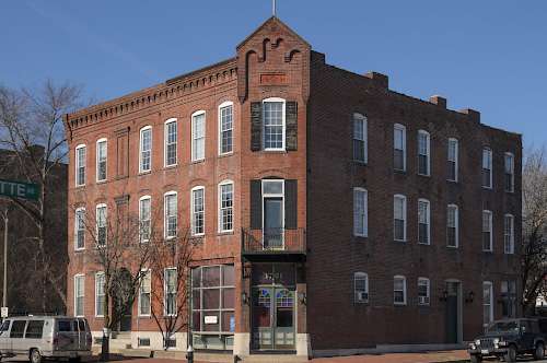
A building in the Soulard neighborhood, in Saint Louis, Missouri, USA.
By modern standards, this is a very small image. It is 500 pixels across by 332 pixels in height; and if we multiply them together, 500 x 332 = 166,000 total pixels. If we divide that by one million, we get a tiny 0.166 megapixels, a mere 1% or so of the total number of pixels that might be found in a contemporary camera. Don’t get me wrong — all the extra megapixels in my camera did find a good use, for when I made this image by downsampling, some of the impression of sharpness of the original image data did eventually find its way into this tiny image — if I only had a 0.166 megapixel camera, the final results would have been softer.
OK, it is very important to know that a digital image has ultimately a fixed pixel size, and if we enlarge it, we don’t get any more real detail out of it, and if we reduce it, we will we lose detail. Many beginners, if they get Photoshop or some other image editing software, will get confused over image sizes and the notorious “pixels per inch” setting, as we see in this Photoshop dialog box:
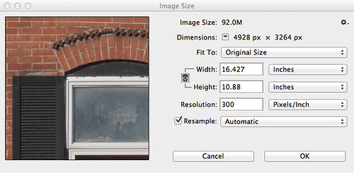
If you are displaying an image on the Internet, the “Resolution” or “Pixels/Inch” setting is meaningless because the image will display on the monitor at whatever the resolution of the display happens to be set at. Likewise, if you make a print, the Width and Height values you see here are likewise meaningless, for the dimensions of the printed image will be whatever size the image is printed at — and not these values. But — if you multiply the Pixels/Inch value by the Width or Height, you will get the actual pixel dimensions of the image.
The really important value then is the pixel dimensions: my camera delivers 4928 pixels across and 3264 pixels in the vertical dimension. I can resample the image to have larger pixel dimensions, but all those extra pixels will be padding, or interpolated data, and so I won’t see any new real detail. I can resample the image smaller, but I’ll be throwing away detail.
Sensels and Pixels
So, we might assume that my camera’s sensor has 4,928 pixels across and 3,264 pixels vertically — well, it actually has more than that, for a reason we’ll get to later. But in another sense, we can say that the camera has fewer pixels than that, if we define a pixel as having full color information. My camera then does not capture whole pixels, but only a series of partial pixels.
It would be more correct to say that a 16 megapixel camera actually has 16 million sensels, where each sensel captures only a narrow range of light frequencies. In most digital cameras, we have three kinds of sensels, each of which only captures one particular color.
The image sensor of my particular model of Nikon has a vast array of sensels — a quarter of which are only sensitive to red light, another quarter sensitive to blue light, and half sensitive to green light, arrayed in a pattern somewhat like this one:
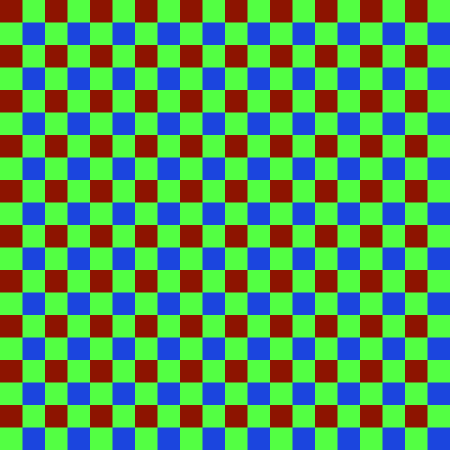
Since I was unable to find a good photomicrograph of an actual camera sensor, this will have to do for our needs — but this abstract representation doesn’t really show us the complexity of sensors.
Not only is the sensor most sensitive to a bright yellowish-green light (as far as I can tell), it has less sensitivity to blue, and is less sensitive to red: this is on top of the fact that we have as many green sensels as we have red and blue combined. Please be aware that the camera can only deliver these colors (in a variety of brightnesses), and so somehow we are going to have to find some means of combining these colors together in order to get a full gamut of color in our final image.
We have information on only one color at each sensel location. If we want to deliver a full pixel of color at each location, we need to use an interpolation algorithm — a method of estimating the full color at any particular sensel location based on the surrounding sensels. This process of estimating colors is called demosaicing, interpolation, or debayering — converting the mosaic of colors to a continuous image.
Camera raw files are of great interest because they record image data that have not yet been interpolated; you can, after the fact on your computer, use updated software that might include a better interpolation algorithm, and so you can possibly get better images today from the same raw file than what you could have gotten years ago.
Please be aware that the kind of pattern above — called a Bayer filter, after the Eastman Kodak inventor Bryce Bayer (1929–2012) — is not the only one. Fujifilm has experimented with a variety of innovative patterns for its cameras, while the Leica Monochrom has no color pattern at all, since it shoots in black and white only. Also be aware that the colors that any given model of camera captures might be somewhat different from what I show here — even cameras that use the same basic sensor might use a different color filter array and so have different color rendering. Camera manufacturers will use different formulations of a color filter array to adjust color sensitivity, or to allow for good performance in low light.
Sigma cameras with Foveon X3 sensors have no pattern, since they stack three different colors of sensels on top of each other, giving full-color information at each pixel location. While this may seem to be ideal, be aware that this design has its own problems.
A Clarification
I am using the term ‘color’ loosely here. Be aware that many combination of light frequencies can produce what looks like — to the human eye — the same color. For example, a laser might produce a pure yellow light, but that color of yellow might look the same as a combination of red and green light. This is called metamerism, and is a rather difficult problem. There are any number of formulations of color filters that can be used in a digital camera, and we can expect them to have varying absorbance of light — leading to different color renderings. For this reason, it is difficult to get truly accurate colors from a digital camera.
A Perfect Sample Image
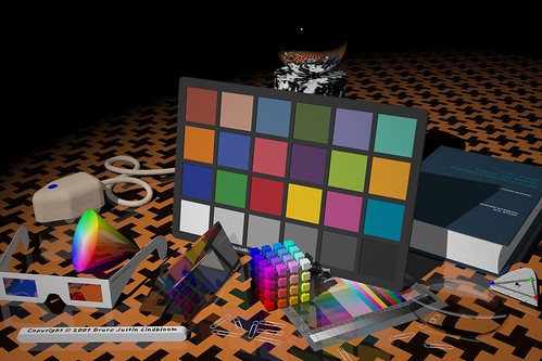
For my demonstrations of demosaicing, I’ll be using sections of this image (Copyright © 2001 by Bruce Justin Lindbloom; source http://www.brucelindbloom.com):
Mr. Lindbloom writes:
In the interest of digital imaging research, I am providing a set of four images that represent "perfect" images, that is, they represent a natural scene (as opposed to say, a test pattern or a gradient) which is completely void of any noise, aliasing or other image artifacts. They were taken with a virtual, six mega-pixel camera using a ray tracing program I wrote myself. The intensity of each pixel was computed in double precision floating point and then companded and quantized to 8- or 16-bits per channel at the last possible moment before writing the image file. The four variations represent all combinations of 8- or 16-bits per channel and gamma of 1.0 or 2.2. I believe these images will be useful for research purposes in answering such questions as "How many bits are needed to avoid visual defects?" and "How does one determine the number of bits of real image information, as opposed to digitized noise?" In this sense, they may provide ideal image references against which actual digitized images may be compared by various visual or statistical analysis techniques.No camera — at the same resolution — will produce images as sharp as this, nor will any camera produce colors as accurate as this image, and no camera image will be without noise. Using perfect images for our purposes has the benefit that it will make defects more visible; real cameras will have less pristine images.
I am using two small crops of this image, 100x150 pixels in size each, which I show here enlarged 500%:
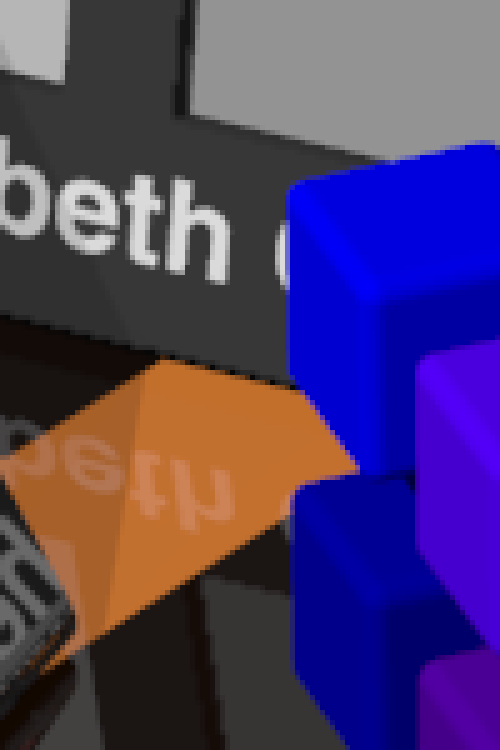

Applying the Mosaic
The sample image has brilliant, saturated colors of impossible clarity. But what happens if we pretend that this image was taken with a camera with a Bayer filter? Here I combine the image crop with a red-green-blue array similar to the one shown above:

It looks rather bad, and recovering something close to the original colors seems to be hopeless. What is worse, we apparently have lost all of the subtle color variations seen in the original image. If we take a closer look at this image:
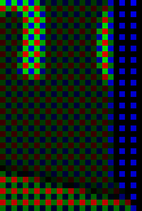
We see that we have only three colors [technically the red, green, and blue primary colors of the sRGB standard] with only variation in brightness. We seemed to have lost much of the color of our original image.
But this is precisely what happens with a digital camera — all the richness and variety of all the colors of the world get reduced down to only three colors. However, all is not lost — if we intelligently select three distinct primary colors, we can reconstruct all of the colors that lay between them by specifying varying quantities of each primary. This is the foundation of the RGB color system. Please take a look at these articles:
Removing the Matrix
Now we have lost color information because of the Bayer filter, and for most digital cameras we simply have to accept that fact and do the best we can to estimate the color information that has been lost. Since each pixel or rather sensel only delivers one color — and we need three for full color — we can have to estimate the colors by looking at the neighboring sensels and making some assumptions about the image. Red sensels need green and blue color data, green sensels lack red and blue data, and blue sensels need red and green.
A very simple method for doing this is the Nearest Neighbor interpolation algorithm, where we grab adjacent sensel colors and use those to estimate the full color of the image. Here is an illustration of a nearest neighbor algorithm:

Take a look at the three original color channels — in the red, we only have data from the red sensel, and the rest are black — and so we copy that red value to the adjoining sensels. Since we have two different green sensels, here we split the difference between them and copy the resulting average to the red and blue sensels. We end up with a variety of colors when we are finished. Now there are a number of ways we can implement a nearest neighbor algorithm, and these depend on the arrangement of the colors on the sensor, and each one will produce somewhat different results.
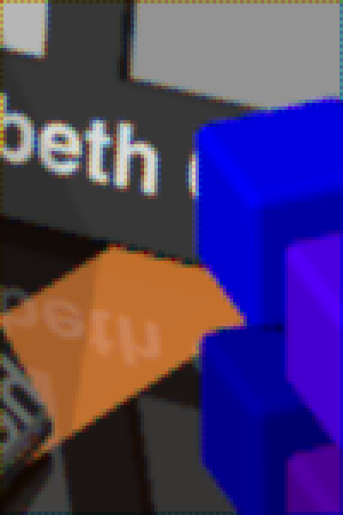
Here we apply a nearest neighbor algorithm to our sample images:
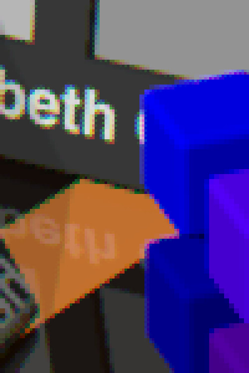
OK, it is apparent that we can reproduce areas of uniform color well, giving us back the colors of the original image. However, edges are a mess. Since the algorithm used has no idea that the lines on the second image are supposed to be gray, it gives us color artifacts. Generally, all edges are rough. Also notice that there is a bias towards one color on one side of an object, and a bias towards another color on the other side of the same object — in the samples, the orange patches have green artifacts on its top and left edges, and red artifacts on its bottom and right edges. This bias makes sense since we are only copying color data from one side of each sensel.
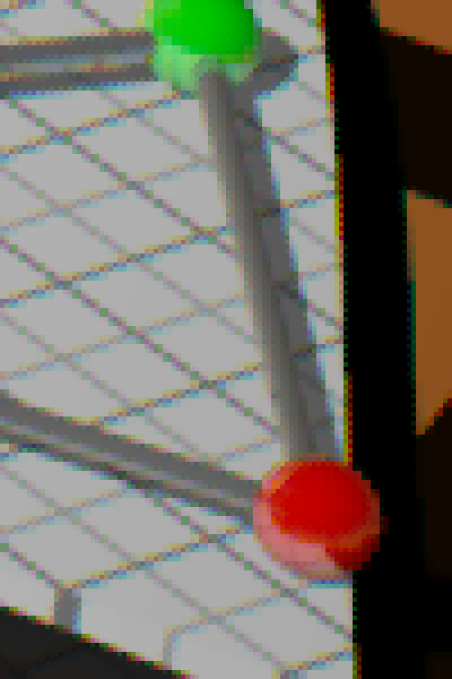
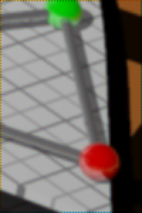
We can eliminate this bias if we replace the Nearest Neighbor algorithm with something that is symmetric. A Bilinear algorithm will examine the adjacent colors on all sides of each sensel, getting rid of the bias. Our sample images here are demosaiced with a bilinear algorithm:

OK, a bilinear algorithm eliminates the directional bias of color artifacts, which is good. While the edges are still rough, they do seem a bit softer — which makes sense, since we are taking data from a wider range of sensels, which in effect blurs the image a bit.
Demosaicing algorithms all assume that colors of adjacent pixels are going to be more similar to each other than they are different — and if we cannot make this assumption, then we can’t do demosaicing. Nearest neighbor algorithms assume that all colors in a 2x2 block are basically identical, while the bilinear algorithm assumes that colors change uniformly in a linear fashion. If we sample sensels farther away, we can assume more complicated relationships, such as a power series, and this assumption is built into the bicubic algorithm, which produces smoother results than those illustrated.
More complex algorithms will give us better gradations and smoothness in color, but have the side-effect of softening edges, and so there is research in ways of discovering edges to handle them separately, by forcing colors along an edge to one value or another. Some algorithms are optimized for scanning texts, while others are better for natural scenes taken with a camera. Be aware that noise will change the results also, and so there are some algorithms that are more resistant to noise, but may not produce sharp results with clean images.
As high frame rates are often desired for cameras, complex algorithms for producing JPEGs may not be desired, simply because it will take much longer to process each image — however, this is less of a problem with raw converters on computers, since we can assume that a slight or even long delay is more acceptable.
Notice that our bilinear images have a border around them. Because the bilinear algorithm takes data from all around each sensel, we don’t have complete data for the sensels on the edges, and so there will be a discontinuity on the border of the image. Because of this, cameras may have slightly more sensels than what is actually delivered in a final JPEG — edges are cropped.
We ought not assume that a camera with X megapixels needs to always deliver an image at that size: perhaps it makes sense to deliver a smaller image? For example, we can collapse each 2x2 square of sensels to one pixel, producing an image with half the resolution and one quarter the size, and possibly with fewer color artifacts. Some newer smartphone cameras routinely use this kind of processing to produce superior images from small, noisy high-megapixel sensors. This is a field of active research.
Antialias
Don’t pixel peep! Don’t zoom way into your images to see defects in your lens, focus, or demosaicing algorithms! Be satisfied with your final images on the computer screen, and if you make a large print, don’t stand up close to it looking for defects. Stand back at a comfortable distance, and enjoy your image.
Perhaps this is wise advice. Don’t agonize over tiny details which will never be seen by anyone who isn’t an obsessive photographer. This is especially true when we routinely have cameras with huge megapixel values — and never use all those pixels in ordinary work.
But impressive specifications can help you even if you never use technology to its fullest. If you want a car with good acceleration at legal highway speeds, you will need a car that can go much faster — even if you never drive over the speed limit. If you don’t want a bridge to collapse, build it to accept far more weight than it will ever experience. Most lenses are much sharper when stopped down by one or two stops: and so, if you want a good sharp lens at f/2.8, you will likely need to use an f/1.4 lens. A camera that is tolerable at ISO 6400 will likely be excellent at ISO 1600. If you want exceptionally sharp and clean 10 megapixel images, you might need a camera that has 24 megapixels.
OK, so then let’s consider the rated megapixel count of a camera as a safety factor, or as an engineering design feature intended to deliver excellent results at a lower final resolution. Under typical operating conditions, you won’t use all of your megapixels. As we can probably assume, better demosaicing algorithms might produce softer, but cleaner results, and that is perfectly acceptable. Now perhaps those color fringes around edges are rarely visible — although resampling algorithms might show them in places, and so getting rid of them ought to be at least somewhat important.
My attempts to blur the color defects around edges was not fruitful. In Photoshop, I attempted to use a half dozen methods of chroma blur and noise reduction, and either they didn’t work, or they produced artifacts that were more objectionable than the original flaws. The problem is, once the camera captures the image, the damage is already done: the camera does in fact capture different colors on opposite sides of a sharp edge — a red sensel might be on one side of an edge, and the blue sensel captures light from the other side.
In order to overcome unpleasant digital artifacts, most cameras incorporate antialias filters: they blur the image a bit so that light coming into the camera is split so that it goes to more than one sensel. This process can only be done at the time of image capture, it cannot be duplicated in software after the fact. Since I am working with a perfect synthetic image, I can simulate the effect of an antialias filter before I impose a mosaic.
Here I used box blur, at 75% opacity on the original image data before applying the mosaic: demosaicing leads to a rather clean looking image:

Now I could have used a stronger blurring to get rid of more color, but I think this is perfectly adequate. What little color noise that still remains can be easily cleaned up by doing a very slight amount of chroma noise reduction — but it is hardly needed. If I would have used stronger blurring, the residual noise would have been nearly non-existent, but it would also have made the image softer. Note that we still have the border problem, easily fixed by cropping out those pixels.
It is typically said that the purpose of the antialias filter is to avoid moiré patterns, as illustrated in the article The Problem of Resizing Images. Understand that moiré patterns are a type of aliasing — in any kind of digital sampling of an analog signal, such as sound or light, if the original analog signal isn’t processed well, the resulting digital recording or image may have an unnatural and unpleasant roughness when heard or seen. From my experience, I think that avoiding the generation of digital color noise defects due to the Bayer filter is a stronger or more common reason for using an antialias filter. But of course, both moiré and demosaicing noise are examples of aliasing in general, so solving one problem solves the other.
Producing a good digital representation of an analog signal requires two steps: blurring the original analog signal a bit, followed by oversampling — collecting more detailed data than you might think you actually need. In digital audio processing, the original analog sound is sent through a low-pass filter, eliminating ultrasonic frequencies, and the resulting signal is sampled at frequency more than double the highest frequency that can be heard by young, healthy ears — but this is not wasteful but rather essential for high-quality digital sound reproduction. Likewise, high megapixel cameras — often considered wasteful or overkill — ought to be seen as digital devices which properly implement oversampling so as to get a clean final image.
Anti-antialias
There has been a trend in recent years of DSLR camera makers producing sensors without antialias filters. A common opinion of this practice is that it makes for sharper-looking images. Indeed they are sharper looking — compare our images that implement the nearest neighbor algorithm with those which are blurred at the bottom. But is that apparent sharpness due to aliasing — a defect of processing — and isn’t real detail at all?
So in some respects, getting rid of an antialias filter ought to be considered a mistake. Perhaps Nikon realizes this, offering both the D800, which incorporates an antialias filter, and the D800E, which incorporates another filter which cancels out the effect of the antialias filter. But be aware that there is no way to digitally correct for the loss of the antialias blurring step of the original analog signal. Any attempts, after the fact, to correct for the digital aliasing flaws, will inevitably be worse than if the analog signal was blurred to begin with.
However, practically speaking, it is extremely difficult to get a pixel-level sharp image from a high megapixel camera, especially when the camera is a small image format like DSLRs. Optics usually aren’t all that good and excellent optics are often rare. Also, camera shake, poor focus, narrow depth of field, and diffraction will all blur the light hitting the sensor, giving us the analog pre-blur that is needed to produce clean digital images. In this case, elimination of the antialias filter can actually provide truly sharper images — since we don’t want to further blur light that is already blurry enough to avoid artifacts.
Be aware that construction of an antialias filter is rather problematic and they are not necessarily mathematically perfect for the purpose of pre-blurring the analog light signal for the Bayer filter. We do find a wide variation of anti-alias filters in various camera models, with some having the reputation of being too strong than needed.
Some Further Notes
A quick Web search for “demosaicing algorithms” will bring up many scholarly articles regarding the strengths and weaknesses of the various methods of interpolation, but these are rarely of interest to a photographer.
What a photographer needs to know is that the process does exist, and that most of the time, the method used isn’t too particularly important. The results and artifacts produced by demosaicing only become critical to image quality when the photographer is trying to do something extreme — like making tiny crops of an image or producing huge images, where exceptional optics are used with refined technique: where there is a real need to produce the cleanest possible images. This might also be useful if you are using a low-resolution camera with sharp optics. Otherwise, for casual photography, the details of demosaicing are of little value. Sometimes we simply need to retouch out obvious defects, like blurring the color along particularly noxious edges.
Most raw converter software does not give us any choice in demosaicing algorithm. But some that do include Raw Photo Processor, dcraw, darktable, and RawTherapee. The latter is interesting because you can quickly see the results of changing the algorithm used.
Logically, I am presenting demosaicing as the first step in processing a raw file, but this is not necessarily the best thing to do — I am simply describing it now to get it out of the way. The Dcraw tutorial demonstrates that white balance ought to be done before demosaicing, otherwise additional color artifacts might be generated.
Click here for the previous article in the series:
Cook Your Own Raw Files, Part 1: Introduction
And the next article:
Cook Your Own Raw Files, Part 3: Demosaic Your Images
No comments:
Post a Comment